Anyone who has set up an RTK receiver on a known point and watched the coordinate display has noticed something that can feel unsettling at first. The position is constantly updating and changing. The receiver is fixed nothing is moving but it never quite settles on a single position. Each shot is affected by small changes in satellite geometry, atmospheric conditions, signal noise, and reflected signals from nearby objects. Most of these errors are tiny but they add up causing the RTK position to form a small cluster around the true point instead of landing on the true point itself. The important question you should be asking is “How much movement is normal” not “why is my RTK shot not perfect”.
Why RTK Error forms a Pattern
How to Read an RTK Accuracy Spec
Real Data: Hemisphere S631 on a Surveyed Monument
Why the Bell Curve Matters
A Note on Artificial GPS Error
What This Means for Field Practice
To understand how RTK error works it helps to first understand the statistics used to quantify the accuracy of the receiver.
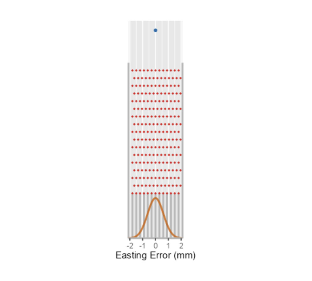
Every RTK observation is affected by small sources of error that will add up and move the calculated position around. The error might push the position slightly north and another might push it slightly south. With enough observations taken, a bell curve will begin to form centered around the true point with more observations close and less far away. Take a plinko board as example, each individual chip can land anywhere but the more chips that are dropped they will begin to form a normal distributed bell curve near the center of the board.
A plinko board shows how many small random events can combine into a predictable bell-shaped normal distribution. RTK error behaves in a similar way as one position may vary slightly, but many positions form a cluster around the true coordinate. RTK observations forming a normal distribution is crucial as it allows for statistical analysis method that only work for normal distributions.
The general format for RTK accuracy found in datasheets is of the form “8 mm + 1 ppm”. This seems simple but understanding this single term can give you more accurate results out in the field. The 8 mm is the base accuracy this describes the expected error under normal conditions. The 1 ppm is a distance-based term describing how the accuracy changes as distance from the correction source grows. Ppm stands for parts per million which in this case means for every kilometer of distance between the base and rover 1 mm of uncertainty is added.
How ppm Affects the Total Error
| Baseline Distance | Added Error at 1 ppm | Total Error |
| 0 km | 0 mm | 8 mm |
| 5 km | 5 mm | 13 mm |
| 10 km | 10 mm | 18 mm |
| 20km | 20 mm | 28 mm |
The reason for this error is that the farther the base and rover are away from each other the larger the difference of atmospheric conditions between those two areas. So, a rover working 2 km away from the correction source will not have the same budget as a rover working 30 km away.
The last part of the accuracy spec is RMS which stands for Root mean Square. This value represents the typical size of the error across many observations by taking the error in the northing or easting and take it to the power of two so that the direction of the error has no effect. This means that a 2 cm error in the north and a 2 cm error in the south will not cancel out. The formula used to calculate this is:
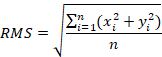
This formula squares all of the errors (e) and then sums them, divides by the total number of observations (n) and then square roots that fraction. There are more RTK accuracy measurements that sound similar in name but are looking at accuracy differently. These are DRMS, 2DRMS, and R95. DRMS is the Distance Root Mean Square and in this case represents the horizontal error by creating a radius of the main horizontal error cluster. The DRMS formula is as follows with x as easting error and y as northing error.
2DRMS as the name suggests is simply the DRMS value multiplied by 2 and gives the radius of an approximate 95% horizontal confidence interval. A confidence interval is how confident we can be that a percentage of positions will land within a certain radius of the receiver. So lets say 100 shots are taken we are confident at least 95 of those shots land within the 2DRMS radius. The R95 is the actual radius that contains 95% of the recorded positions. Quick recap after lots of information, the RMS describes the size of the error while DRMS, 2DRMS, and R95 describe that error as a radius around the true point. The important takeaway from this information is that an RTK accuracy spec is not a promise that every shot will be exactly that close. It is a statistical description of how the position should cluster under normal conditions.
To see how this looks in practice, a Hemisphere S631 was set up on a surveyed monument with known coordinates. The receiver was connected to our StormCaster network and recorded 600 auto-recorded points at one-second interval. The pole was leveled and then untouched and the receiver stayed fixed the entire time. The horizontal results are seen in the plot below.
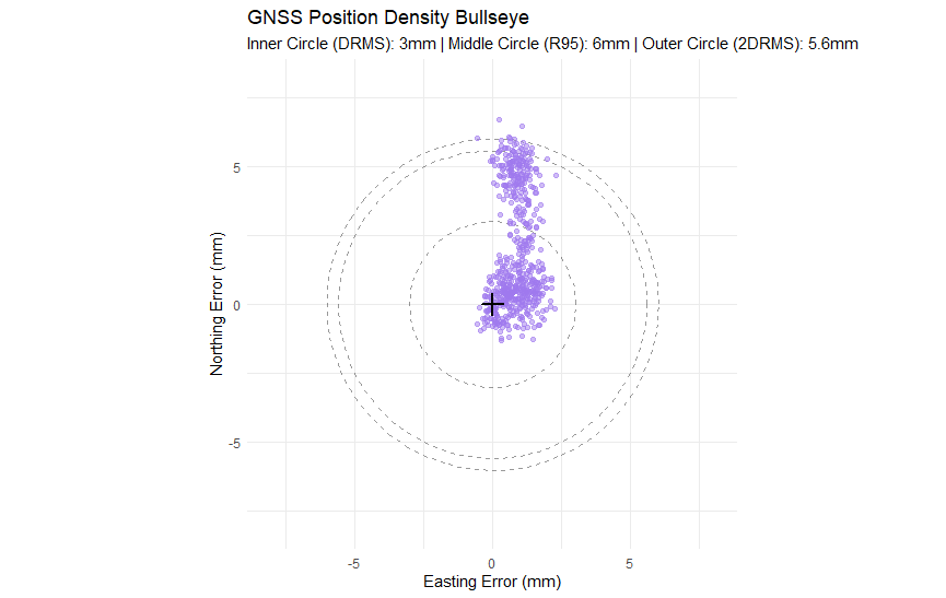
Figure 1: Scatter plot of 600 RTK positions recorded on a surveyed monument. Each mark represents one recorded position. The centre point is the true monument coordinate. The inner circle shows the measured DRMS of 3mm, the middle circle shows the R95 value which means 95 % of the points landed within 5.6 mm and the outer circle is the 2DRMS which is 6 mm.
Some information not given on the horizontal plot is there was a mean horizontal error of 2.405 mm, a standard deviation in northing error of 2.126 mm and a standard deviation in easting error of 0.539 mm. The height data followed the same general pattern with an average height error of -1.16 mm indicating on average it was saving its position slightly lower than the true height. The standard deviation was 1.36 mm indicating a tightly grouped cluster around the average.
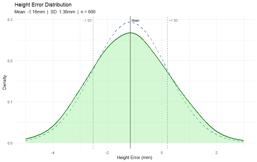
Figure 2: Height error distribution from 600 RTK observations. The green curve shows the measured height errors. The dashed blue line shows a theoretical normal distribution using the same mean height error of -1.16 mm and standard deviation of 1.36 mm. The close match shows that the height errors follow a predictable statistical pattern
The height results follow the same pattern as the horizontal positions. Most of the heights are tightly grouped near the average height error of -1.16 mm. That means the receiver was measuring slightly low on average, but only by a very small amount. The standard deviation was 1.36 mm, which shows that the height observations were very closely clustered. In other words the receiver was producing a consistent height solution with small variation around the mean. The dashed blue line is a reference normal distribution based on the measured mean and standard deviation. Since the measured height data closely follows that curve, it supports the idea that RTK error behaves in a predictable statistical pattern rather than random scatter.
The bell curve matters because it gives us a practical way to describe RTK accuracy. When errors follow a normal distribution, most observations land close to the average, and fewer observations land farther away this allows us to use confidence levels to describe how much movement is normal. For a normal distribution, about 68% (68.27%) of observations fall within one standard deviation of the mean. About 95% (95.45%) fall within 2 standard deviations. These percentages are not exact for each individual shot but they describe what we expect to happen across many observations. That is why terms like RMS, DRMS, 2DRMS, and R95 are useful. They do not promise that every shot will land in the exact same place, they describe how tightly the shots should cluster around the true point. In simple terms, the bell curve is what lets us turn a moving RTK position into a measurable accuracy statement.
Older GPS included a feature called Selective Availability, which intentionally reduced civilian GPS accuracy. Selective availability was turned off in 2000, so it is not the reason modern RTK positions move around the true position. Modern GNSS still has error but it is not “artificial” in the same sense. Artificial error can still be found today from jamming, spoofing, interference, or poor correction data being introduced into the system. Most RTK scatter comes from real measurement conditions: atmosphere, multipath, receiver noise, satellite geometry, baseline length, and field setup. There are small signal errors in modern GNSS like satellite clock error, orbit error, signal biases, and timing uncertainty. These are not intentional errors added to the signal but the limitations of measuring time and distance from satellites moving thousands of kilometers away.
Under favourable conditions with a nearby correction source and good satellite geometry, a quality RTK receiver will routinely deliver performance well inside its stated specification. The 3mm DRMS result above reflects what the hardware is capable of under good but genuine outdoor conditions, rather than what you should expect on every setup during a full day of survey work.
The distance-dependent term deserves more attention than it typically receives. At short baselines it is easy to ignore, but at 20 or 30km it begins to consume a meaningful portion of the RTK error budget. A surveyor working 30km from the nearest correction source is carrying a fundamentally different specification than the headline figure on the box, and field decisions should reflect that.
Finally, it is worth remembering that the 8mm RMS figure is an absolute value in both directions. It describes the standard deviation from the mean, meaning observations can fall up to 8mm in any direction from the true position, not 4mm in total. The full expected spread at one standard deviation is 8mm either side of centre. For tight-tolerance applications this distinction matters, and it is one reason why understanding the statistical meaning of the spec, rather than simply noting the number, leads to better professional decisions in the field.
